After I shared our article about testing SmolBox with nested KVM, a reader asked about performance. They had seen reports of large overhead from nested virtualization but had never measured it themselves.
Neither had I. We chose nesting so we could deliberately break a disposable worker environment and recover it from the physical host. It gave us a place to test full disks, worker failures and an unresponsive outer VM.
Their question was worth an experiment. On the same Linux machine, I compared a microVM running directly on the host with one running inside our lab VM.
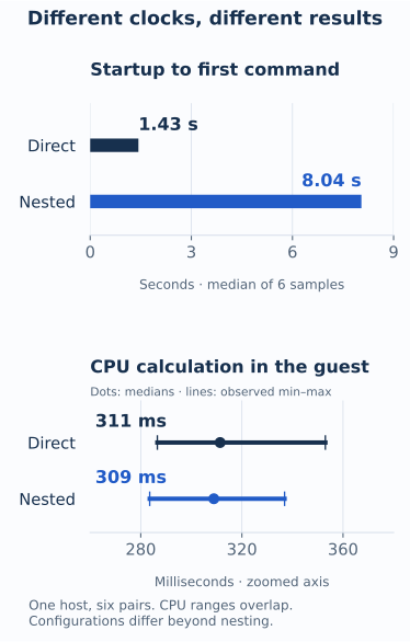
Startup was much slower in the nested setup. The short CPU calculation had overlapping timings. Both observations matter when someone asks how much overhead nesting adds.
One question, several clocks
SmolBox manages disposable smolvm executions from Elixir. It tracks the job, collects its output and keeps cleanup visible until it finishes. SmolBox itself does not require nested virtualization.
For a program already running, overhead means extra time doing its work. For an application submitting a new job, it also includes creating the machine, starting it, transferring files and collecting the result. The capacity stays occupied until cleanup completes.
I measured those intervals separately. Otherwise, a large startup penalty could be mistaken for an equally large slowdown in every instruction the guest runs.
Same workload, an extra layer
Both configurations used the same smolvm binaries, approved Python image and microVM allocations. The Elixir controller ran beside its worker and used a private Unix socket in each case.
| Component | Configuration |
|---|---|
| Physical Linux host | Intel Core i5-1135G7, 4 cores / 8 threads, 64 GiB RAM |
| Outer VM for the nested tests | 4 vCPUs, 8 GiB RAM |
| Each tested microVM | 1 vCPU, 512 MiB RAM |
| Software in both configurations | SmolBox 0.1.3, smolvm 1.16.0, Python 3.12.14 |

I ran one warmup per configuration, then six measured pairs, alternating which configuration went first. Each sample created fresh machines. Images were already prepared and disk templates decompressed; downloads and dependency installation were outside the timings. Host caches were warm.
The workloads were deliberately small: a command that immediately exits, a fixed
Python integer calculation, and a 36 MiB file write followed by fsync, a read
and a hash check. A separate managed job followed the file workload through
submission, output collection and verified cleanup.
Where the time went
These results compare two complete deployment configurations, which differ in more than their virtualization layers.
These are medians across six samples per configuration:
| Measurement | Direct | Nested |
|---|---|---|
| Startup to the first successful command | 1.43 s | 8.04 s |
| Tiny command on a running VM, client round trip | 95.6 ms | 91.2 ms |
| CPU calculation inside the guest | 311 ms | 309 ms |
| File processing inside the guest | 179 ms | 442 ms |
| Managed file job through output collection | 2.41 s | 8.90 s |
| Managed file job through verified cleanup | 3.14 s | 9.32 s |
Startup includes creation, start and the first successful command. Its median was about 5.6 times longer in the nested setup. The complete managed job, including cleanup, took about three times as long.
The CPU calculation tells a different story. Direct samples ranged from 287–353 ms; nested samples ranged from 284–337 ms. Those ranges overlap. The slightly lower nested median is not evidence that nesting makes computation faster. Timings for the tiny command overlap too.
There is another useful distinction: the CPU command's median client round trip was 479 ms directly and 568 ms nested. An application can wait longer even when the calculation measured inside its guest takes a similar time.
The file test's nested median was about 2.5 times longer, but direct results varied from 162–498 ms. That slow direct sample remains in the results. Six observations are enough for this first comparison, not a reliable estimate of how long jobs might take in the worst case.
What we can attribute to this setup
Neither worker nor the outer VM recorded CPU throttling during the measured intervals. Neither worker hit its memory limit or recorded an OOM kill. All twelve measured samples completed with correct results and verified cleanup.
Still, these were two deployment configurations, with differences beyond the extra virtualization layer. The physical host and outer guest used different Linux kernels. Nested storage passed through guest ext4 and a QEMU disk overlay; the direct worker used host ext4. Filesystem options differed as well.
CPU frequency remained dynamic, other host services stayed running, and we did not pin workloads to dedicated cores. The file test used buffered I/O and warm caches. We did not measure concurrency, network traffic or large working sets.
The full benchmark report records the ranges, resource controls, source identities and setup corrections. The raw sample data and benchmark scripts let readers inspect the measurements and adapt the method to their own environment.
Could another execution model change the result?
These measurements cover SmolBox's current approach: creating a fresh microVM from a prepared image for each execution. smolvm also supports branching running machines and restoring checkpoints. SmolBox 0.1.3 does not expose those operations, and we have not benchmarked them.
They are worthwhile candidates for another experiment. These results cannot tell us how much time they would save or what additional lifecycle management they would require.
Measure the wait your application cares about
Nesting served its purpose in our failure lab: we could damage the worker environment and recover it independently. The extra startup time was a tradeoff we accepted for those tests.
For an application, the relevant question is how often it pays that cost. A short job in a fresh VM and a long calculation inside a running one have very different timing profiles. Our small CPU test also says little about a workload that spends most of its time on I/O.
Start with your real workload. Measure startup, work, result collection and cleanup separately. The useful number is how long your application waits, and which part of that wait you can change.